The Triviality Norm
Feynman famously said that to a mathematician, anything that was proven was trivial. This statement, while clearly a lighthearted dig at mathematics, it does have a striking ring of truth to it.
Logical Implication
In logic, there is the concept of implication. The idea is that if \(B\) is true whenever \(A\) is true we can say that \(A \implies B\). This makes sense for statements that depend on a variable. For example, we can say that \(x > 2 \implies x > 0\).
However, on the other hand, implication, because it is just a mechanical definition based on the truth values of the inputs and not their relationship to each other, can sometimes lead to ridiculous results. For example, this implication is completely valid:
\[1 = 1 \implies a + b = b + a\]
Which doesn’t seem to make sense: the first is a tautology about equality and the second is a tautology about addition. Additionally, the following statement is true:
\[2 = 3 \implies \text{Fermat’s Last Theorem is False}\]
In both cases (truth implies truth and falsehood implies falsehood) make some degree of sense. However, the final case, falsehood implies truth, is where things start becoming weird:
\[2 = 3 \implies 2 = 2\]
In any case, the fact that implication in logic, unlike implication in language, does not imply (in either sense) a connection between two concepts. In fact, there is no distinction between a simple proof and a more complex one. In other words, using logical implication as a metric, anything that is proven is trivial.
Intuitive Implication
\(\newcommand\rew{\gg}\)
We can define intuitive implication, or a rewrite, as a single logical reduction from a step to another, denoted \(A \rew B\). For example, we have
\[\neg (A \wedge B \wedge C) \rew \neg (A \wedge (B \wedge C)) \rew \neg A \vee \neg (B \wedge C) \rew \neg A \vee (\neg B \vee \neg C) \rew \neg A \vee \neg B \vee \neg C \]
However, this general scheme doesn’t seem to work for more complex theorems. For example (using new lines rather than \(\rew\)),
\[a + 0 = a \wedge a + S(b) = S(a + b) \wedge \text{Induction}\] \[a + 0 = a \wedge a + S(b) = S(a + b) \wedge \text{Induction} \wedge 0 + 0 = 0\] \[a + S(b) = S(a + b) \wedge \text{Induction} \wedge 0 + 0 = 0 \wedge (0 + n = n \implies S(0 + n) = S(n))\] \[\text{Induction} \wedge 0 + 0 = 0 \wedge (0 + n = n \implies 0 + S(n) = S(n))\] \[0 + n = n\]
In general, this strategy doesn’t work well. In reality, a different given statement is used at every step in the process. We can represent this process as:
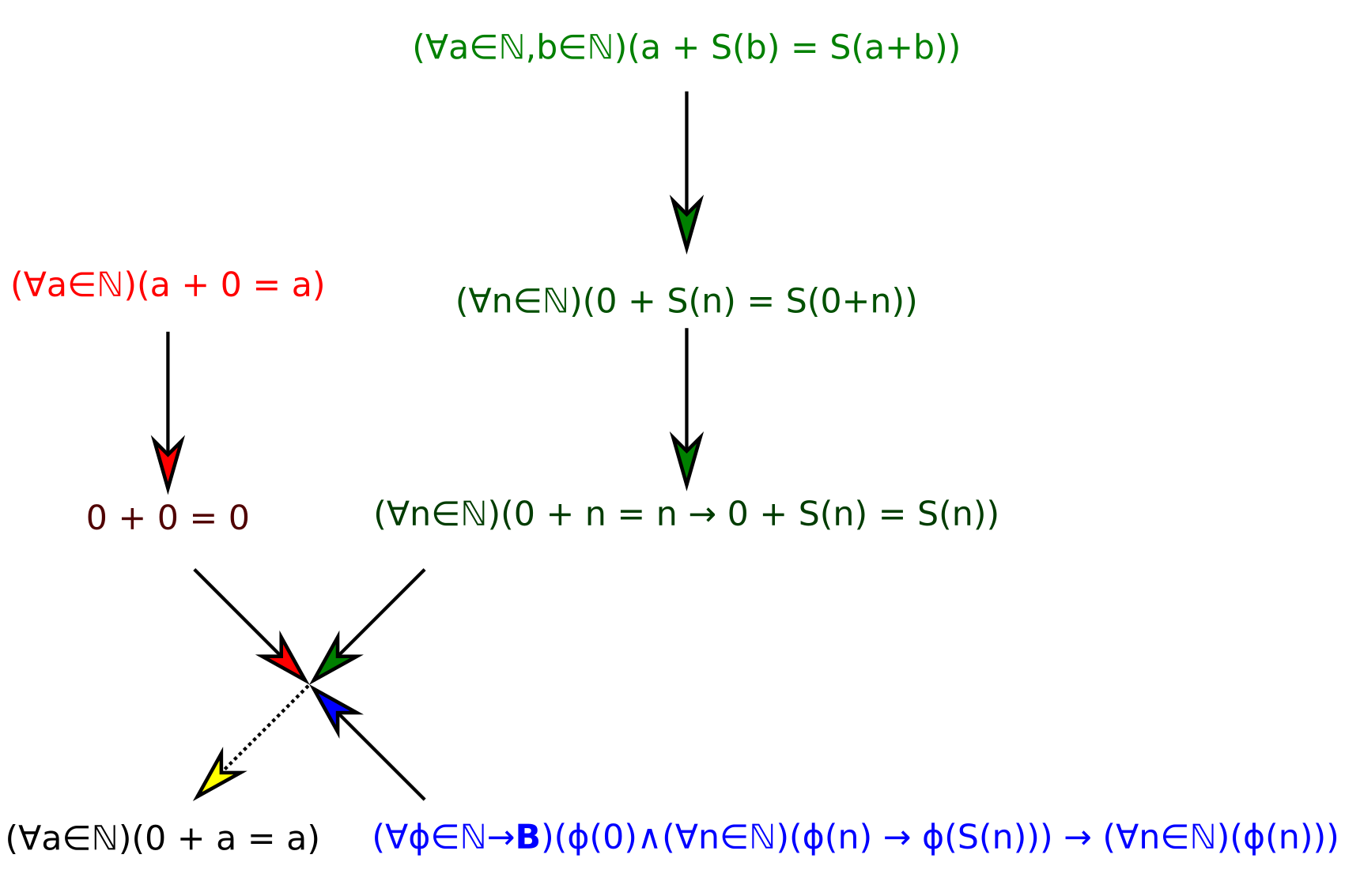
This structure is not exactly a graph, but does have certain properties of one. We can represent each step as an implication between a tuple of statements and a result:
\[(\forall a \in \mathbb N)(a + 0 = a) \rew 0 + 0 = 0\] \[(\forall a \in \mathbb N, b \in \mathbb N)(a + S(b) = S(a + b)) \rew (\forall n\in\mathbb N)(0 + S(n) = S(0+n))\] \[(\forall n\in\mathbb N)(0 + S(n) = S(0+n)) \rew (\forall n\in\mathbb N)(0 + n = n \implies 0 + S(n) = S(n))\] \[\big(0 + 0 = 0;(\forall n\in\mathbb N)(0 + n = n \implies 0 + S(n) = S(n));(\forall\phi\in\mathbb N \to\mathbb B)(\phi(0)\wedge(\forall n\in\mathbb N)(\phi(n) \implies \phi(S(n))) \implies (\forall n \in\mathbb N)(\phi(n)))\big) \rew (\forall n \in \mathbb N)(0 + n = n)\]
The graph structure
The structure of a proof under this scheme is not quite an exact graph. A graph can take the form (using Haskell notation)
data Edge a = Edge {
        from :: a,
        to :: a
    }
data Graph a = Graph [Edge a]
A more convenient representation (for searches, etc.) is:
data GraphNode a = GraphNode {
        value :: a,
        neighbors :: [GraphNode a]
    }

type Graph a = [GraphNode a]
This graph, on the other hand, has asymetrical edges, with multiple start nodes for each end node. We have:
data Edge a = Edge {
        from :: [a],
        to :: a
    }

data Graph a = Graph [Edge a]
A more convenient representation is difficult in this case, given that the transformation used above:
data Neighbor a = Neighbor {
        otherDependencies :: [GraphNode a],
        target :: GraphNode a
    }

data GraphNode a = GraphNode {
        value :: a,
        neighbors :: [Neighbor a]
    }

type Graph a = [GraphNode a]
As you can see, each of the neighbors needs to mantain a list of dependencies, which makes it difficult to see the whole structure of the graph. Instead, we can use edge nodes, making a graph look like this:
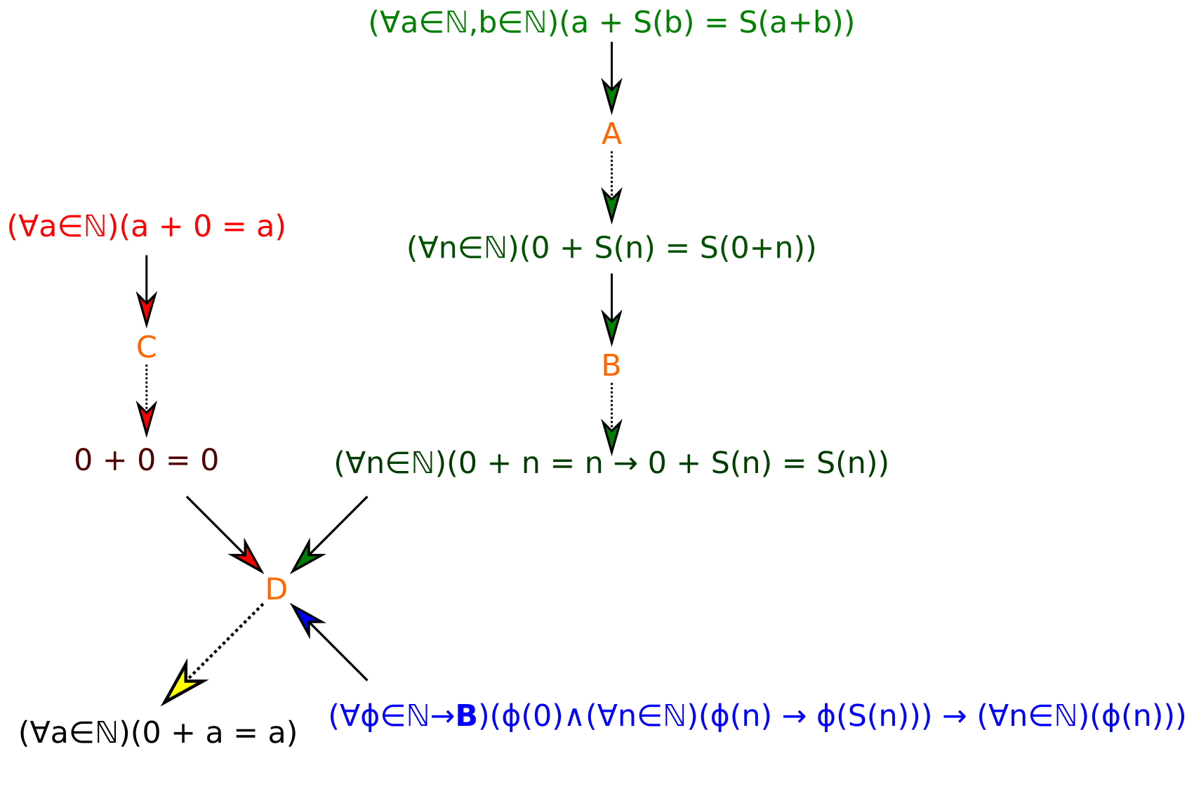
This can be represented like this:
data GraphNode a = GraphNode {
        value :: a,
        contributesTo :: [EdgeNode a]
    }

data EdgeNode a = EdgeNode {
        from :: [GraphNode a],
        to :: GraphNode a
    }

type Graph a = [GraphNode a]
This ends up being a much simpler description, being a traditional graph with two types of nodes and certain restrictions.
The Generalized Levenshtein Distance
The Levenshtein distance, or L-distance, is the minimum number of edits needed to go between two strings, where edits are defined as
- Deleting a character
- Inserting a character
- Replacing a character with another character
One basic generalization is to allow for an arbitrary set of rewrite rules. This is the graph-distance of the rewrite graph, or the graph formed by using statements as nodes and logical conclusions as edges. In this case, a theorem is just two connected nodes, along with the shortest path between them.
However, this fails to take into account the two-node nature of actual proof graphs. In this case, it does not make sense to speak of a path, instead we have a tree with certain leaves, which we know as axioms. The Generalized Levenshtein distance, or GLD, is defined as the number of edges in the tree that lead from a graph node to an edge node. For example, GLD(the above proof that 0 + a = 0 given the Peano Axioms) = 6.
And there you have it, an actual way to measure the triviality of a proof.
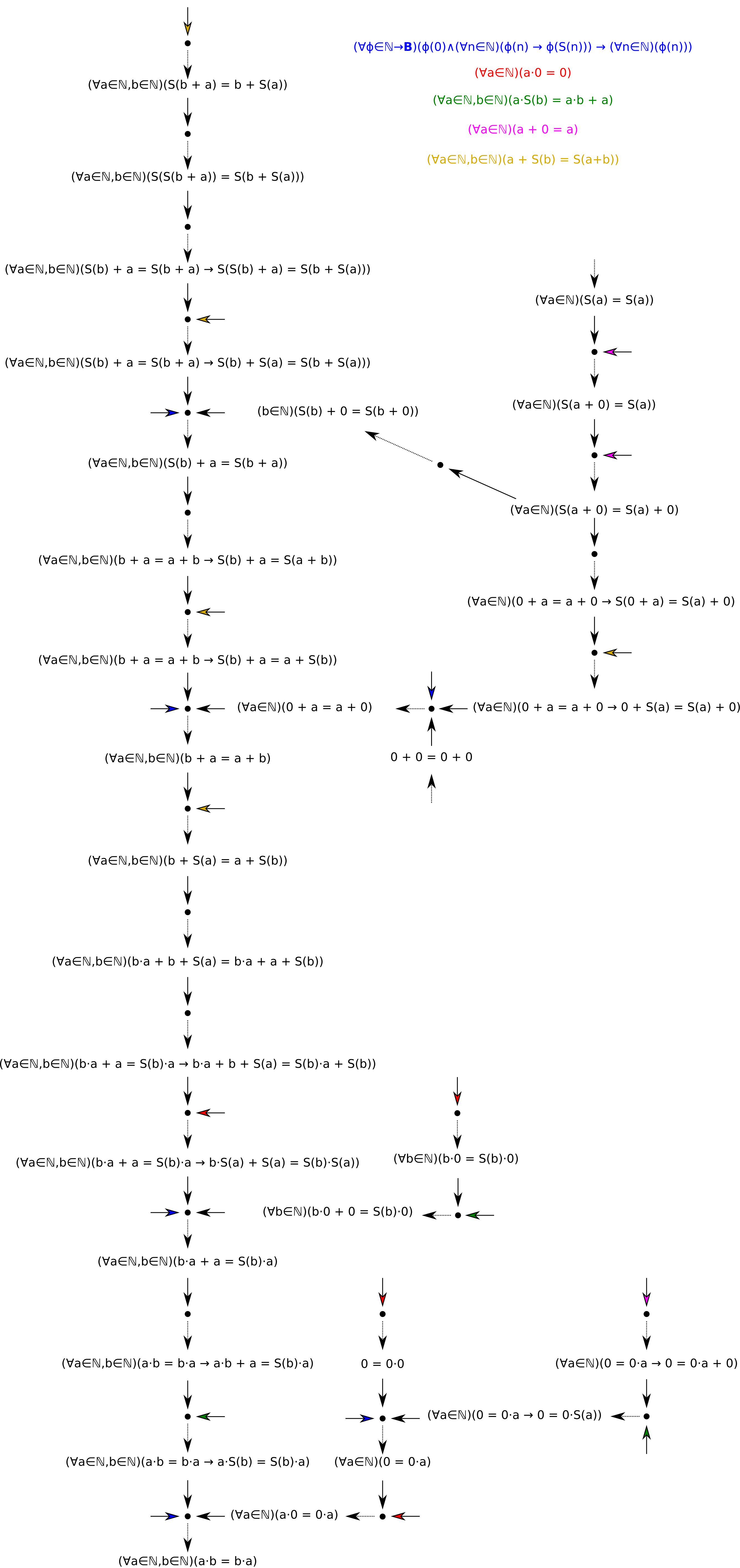
Appendix: A more complex proof
This section isn’t exactly necessary, but drawing complex arrow diagrams is actually pretty fun, so I decided to draw the proof that \(ab = ba\). Note how this proof demonstrates the graph-nature of the proof. (For simplicity, I use colored arrows to refer to axioms, with a color legend at the top.)