Chaos, Distributions, and a Simple Function

\(\newcommand{\powser}[1]{\left{ #1 \right}}\)

Iterated functions

The iteration of a function \(f^n\) is defined as:

\[f^0 = id\] \[f^n = f \circ f^{n-1}\]

For example, \((x \mapsto 2x)^n = x \mapsto 2^n x\).

Most functions aren’t all that interesting when iterated. \(x^2\) goes to \(0\), \(1\) or \(\infty\) depending on starting point, \(\sin\) goes to 0, \(\cos\) goes to something close to 0.739. \(\frac{1}{x}\) has no well defined iteration, as \((x \to x^{-1})^n = x \to x^{(-1)^n}\) which does not converge.

(Note that every convergent value \(x\) satisfies \(f(x) = x\).)

And \(\ln\), no matter where you start, goes to a negative number, which is not in its domain. Of course, we can fix this by squaring its input. Now the iterated function of \(\ln x^2 \) is defined for all \(n\) for any value that isn’t in the set \(0, 1, e, e^{e}, e^{e^{e}}\), etc. That is, almost everywhere. We’ll call this function Iterated Log Square or ITLOGSQ for short.

What does ITLOGSQ look like?

Here’s a plot of ITLOGSQ(n, x) for some \(n\).

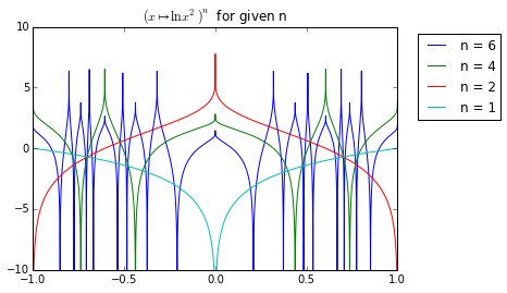
Note how as \(n\) increases, the function gets more complex. In fact, here is ITLOGSQ(10, x):

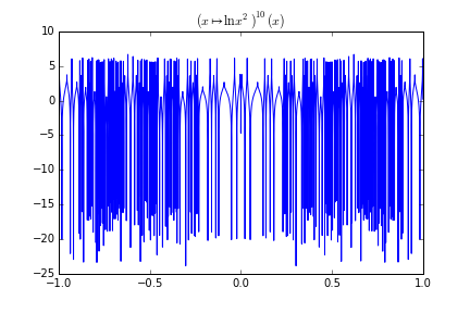
Note specifically how the function erases its input. There seems to be no correlation between input and output. This means that the ITLOGSQ system is chaotic: change the inputs slightly to get a major variation in the output.

The values ITLOGSQ takes

We can look at ITLOGSQ another way: how it distributes its values. For example, here’s what you get if you run a single iteration of ITLOGSQ on a value over and over again, collecting all the results:

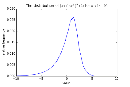
Note the smooth curve. Note that we started at 2 here, but we could have started elsewhere. We can look at the differences between the curves generated at different starting points:

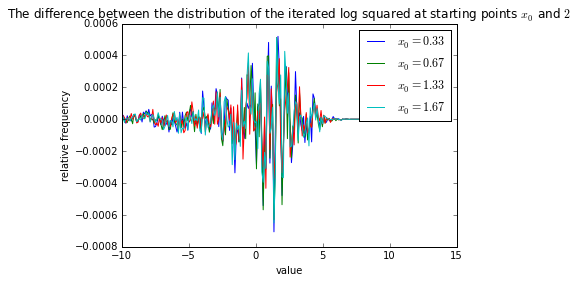
But the differences appear to be mostly random. Also, note that the highest differences are still small compared to the overall size of the actual distributions. In other words, it doesn’t matter what value you start at, the overall distribution is the same.

ITLOGSQ on distributions

What is the distribution of ITLOGSQ(n, x) if \(x\) is described by a uniform distribution? Well, here’s what happens:

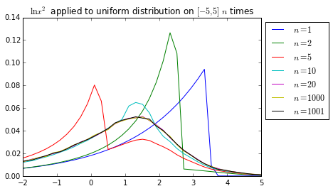
Notice how we can see that the sequence very quickly converges from the fact that the curves for \(n = 20\) and \(n = 1000\) are almost the same. The fact that \(n = 1000\) and \(n = 1001\) are almost the same means that there isn’t a large-scale periodicity.

Interestingly, the limit curve looks a lot like the histogram above. This is no accident: since \(\ln x^2\) is basically uncorrelated with \(x\), randomly selecting numbers and putting a number through the filter over and over again are pretty much the same general idea. Since the sequence converges so quickly, we’re basically sampling the same distribution over and over again for the histogram, therefore, we have similar values.

The distribution of ITLOGSQ(\(\infty\))

Since we know that the distribution of ITLOGSQ converges as \(n\) increases, we know that the convergent distribution \(p\) is a fixed point of the function \(x \mapsto \ln x^2\). This can be expressed as:

\[p(\ln x^2) = \sum_{t | \ln t^2 = \ln x^2} p(t) \] \[p(\ln x^2) = \sum_{t | t^2 = x^2} p(t) \] \[p(\ln x^2) = p(x) + p(-x) \]

With the additional condition (from the fact that this is a probability distribution function):

\[\int_{-\infty}^{\infty} p(x) \text{d} x = 1\]

And I can’t see any way to solve it, but it’s interesting that it can be represented so succinctly.

Code Samples

The code used to generate all of this can be found here. Note that some of the boxes take some time to run.