Haskell Classes for Limits
OK, so the real reason I covered Products and Coproducts last time last time was to work toward a discussion of limits, which are a concept I have never fully understood in Category Theory.
Diagram
As before, we have to define a few preliminaries before we can define a limit. The first thing we can define is a diagram, or a functor from another category to the current one. In Haskell, we can’t escape the current category of Hask, so we instead define a diagram as a series of types and associated functions. For example, we can define a diagram from the category \(\mathbf 2\) containing two elements and no morphisms apart from the identities as a pair of undetermined types.
A diagram from the category \(\mathbf 2*\), a category containing two elements and an arrow in each direction (along with the identities), (this implies that the two arrows compose in both directions to the identitity):
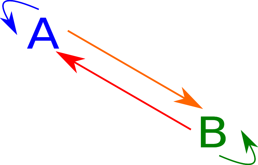
In this case, we have two types A and B as well as two functions of types A -> B and B -> A.
In any case, we can define a diagram of two types as:
data Diagram1 a = Diagram1 [a -> a]
data Diagram2 a b = Diagram2 [a -> a] [a -> b] [b -> a] [b -> b]
data Diagram3 a b c = Diagram3 [a -> a] [a -> b] [a -> c] [b -> a] [b -> b] [b -> c] [c -> a] [c -> b] [c -> c]

twoStarCons :: (a -> b) -> (b -> a) -> Diagram2 a b
twoStarCons f g = Diagram2 [id] [f] [g] [id]
Cones
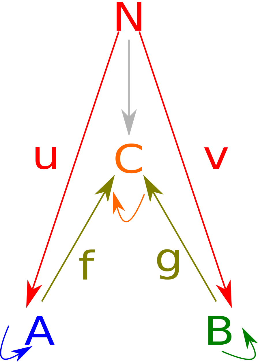
In any case, we can define a cone on a diagram as a set of functions from one element to the image of this diagram. A cone onto a diagram selecting three elements, \(A, B, C\) with six morphisms can be represented as such.
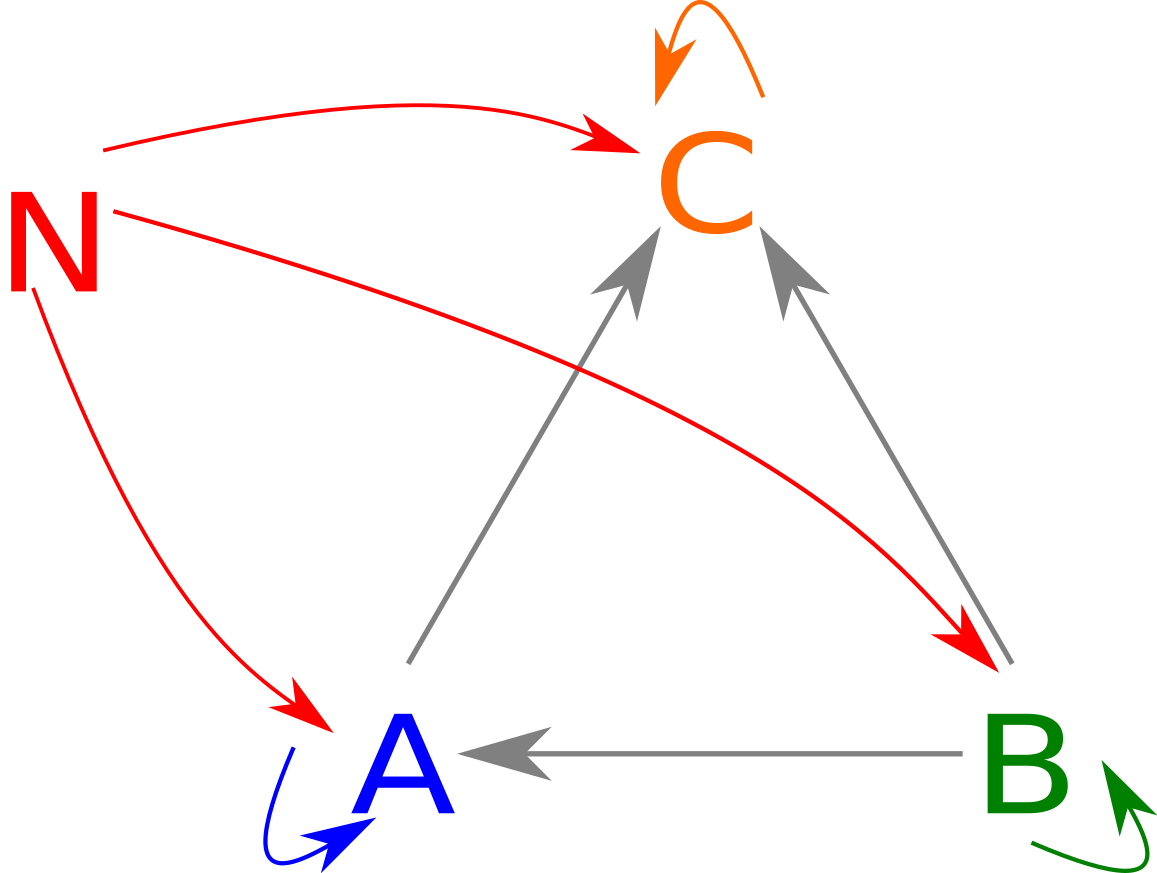
If you imagine \(N\) being above \(A, B, C\) note how the diagram has a roughly conical shape. In fact, for any diagram, you can put all the items in a rough circle and have arrows go along the base, with a whole bunch of triangles along the sides. In Haskell, a cone is represented just by the arrows from \(N\) (traditionally named phi) as such:
class Cone1 n a | n -> a where
    phi1 :: n -> a

class Cone2 n a b | n -> a, n -> b where
    phi2_a :: n -> a
    phi2_b :: n -> b

class Cone3 n a b c | n -> a, n -> b, n -> c where
    phi3_a :: n -> a
    phi3_b :: n -> b
    phi3_c :: n -> c
The cone laws come from the fact that each of the sideways “faces,” i.e., the triangles with two sides being morphisms from \(N\) must commute. One interesting implication is that the only morphism you can have from any object in the diagram to itself can be the identity, otherwise, the “triangle” with both sides being the same doesn’t commute.
cone1Law :: (Cone1 n a, Eq (a -> a)) => Diagram1 a -> Bool
cone1Law (Diagram1 a) = all (== id) a

cone2Law :: forall n a b. (Cone2 n a b, Eq a, Eq b, Eq (a -> a), Eq (b -> b)) => Diagram2 a b -> n -> Bool
cone2Law (Diagram2 aa ab ba bb) n = and [aasat, bbsat, absat, basat]
    where
    f === g = f n == g n
    aasat = all (== id) aa
    bbsat = all (== id) bb
    absat = all (=== phi2_b) $ map (. phi2_a) ab
    basat = all (=== phi2_a) $ map (. phi2_b) ba

-- You get the picture.
Spans and Cones
If you squint a little at the definition of a cone, you can probably see the similarity to a span:
class Span s where
    fst :: s a b -> a
    snd :: s a b -> b
We can in fact make this formality official: anything that is a span is also a cone of a sort:
instance (Span s) => Cone2 (s a b) a b where
    phi2_a = fst
    phi2_b = snd
Of course, satisfying the laws is not as easy. The third part to the law
absat = all (== phi2_b) $ map (. phi2_a) ab
simplifies to
absat = all (== snd) $ map (. fst) ab
which simplifies to
ab_f . fst == snd
being true for any function from A to B in the original diagram. We can quickly disprove the existance of such a function by plugging in (x, y) and (x, y'), where y /= y':
ab_f . fst $ (x, y) == snd (x, y) && ab_f . fst $ (x, y') == snd (x, y')
ab_f x == y && ab_f x == y'
This is obviously nonsense, which means that there can’t two y and therefore B is isomorphic to () or Void. A similar argument can be made to show that A must be isomorphic to () or Void. Therefore, for nontrivial products, we must have no functions from A -> B or back: in other words we have to use 2.
More interesting cones
In any case, let’s look at cones of 2*’s diagram, which we know has to be two isomorphic types. A quick definition of isomorphisms is below:
class Iso a b where
    cast :: a -> b
    cocast :: b -> a

isoLaw1 :: (Iso a b, Eq a, Eq b) => a -> b -> Bool
isoLaw1 x y = cast x == y && cocast y == x
In any case, we can define a 2* class as follows:
class (Iso a b) => Twostar a b where

twoStar :: (Twostar a b) => Diagram2 a b
twoStar = twoStarCons cast cocast
And let’s define a standard isomorphism, let’s say \(a + a = 2a\):
instance Iso (Either a a) (a, Bool) where
    cast (Left x) = (x, True)
    cast (Right x) = (x, False)
    cocast (x, True) = Left x
    cocast (x, False) = Right x
We can now try to create a cone onto this specific case of the diagram. Let’s say we want to map from a -> 2a and a -> a + a. Normally, there would be four ways: \a -> ((a, True), Left a), \a -> ((a, False), Left a), \a -> ((a, True), Right a), \a -> ((a, False), Right a). However, because of the cone law, we have to pick corresponding elements. In other words, we only have two possible implementations:
newtype EithMay2Star a = EM2S a
newtype EithMay2Star' a = EM2S' a
instance Cone2 (EithMay2Star a) (Either a a) (a, Bool) where
    phi2_a (EM2S n) = Left n
    phi2_b (EM2S n) = (n, True)

instance Cone2 (EithMay2Star' a) (Either a a) (a, Bool) where
    phi2_a (EM2S' n) = Right n
    phi2_b (EM2S' n) = (n, False)
Limits
In any case, the point of this wasn’t to explain cones, it was to explain limits.
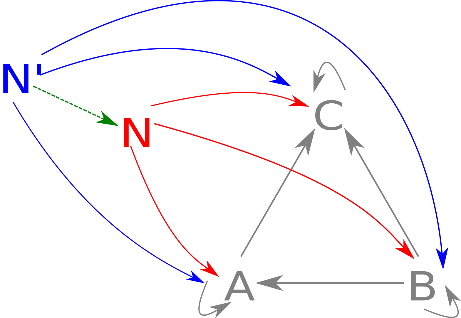
Basically, limits are to cones as proucts are to spans. We say that any other cone can somehow be “factored through” our cone. Here is the limit equivalent of the above cone diagram:
We can represent this as the Haskell class
class (Cone1 n a) => Limit1 n a where
    cFactor1 :: (Cone1 n' a) => n' -> n

class (Cone2 n a b) => Limit2 n a b where
    cFactor2 :: (Cone2 n' a b) => n' -> n

class (Cone3 n a b c) => Limit3 n a b c where
    cFactor3 :: (Cone3 n' a b c) => n' -> n
The sad part is that Haskell’s type system is not advanced enough for us to be able to dewfine all of these as one thing. Anyway, let’s try to think up a limit for 2*.
So, we are given some n', which is the vertex of some cone, so we know that we have an element of a and b. We somehow need to store these and be able to extract them in the implementation of our cone. This sounds like a product. However, we know that in general products won’t do, so we shouldn’t be able to construct one by any means other than cFactor. There’s no real way of enforcing this, so we’ll just make it an abstract data type and never export the constructor.
data Limit2Star a b = L2S a b

instance Cone2 (Limit2Star a b) a b where
    phi2_a (L2S x _) = x
    phi2_b (L2S _ y) = y

instance Limit2 (Limit2Star a b) a b where
    cFactor2 other = L2S (phi2_a other) (phi2_b other)
And since we can only construct using cFactor2, we know that it’s values are always consistent with the underlying diagram.
Pullbacks
OK, so limits are generalized products. But why are they useful? Well, let’s take a walk into the wonderful world that is size 3 diagrams, and look at a fairly simple one: the pullback. It is defined as follows:
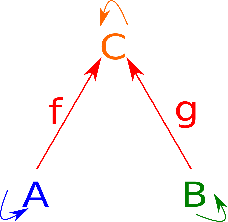
We can represent this as a diagram as follows:
pullbackCons :: (a -> c) -> (b -> c) -> Diagram3 a b c
pullbackCons f g = Diagram3 [id] [] [f] [] [id] [g] [] [] [id]
Looking at a cone over the pullback diagram,
we can notice that any cone over this image is entirely determined by what it sends to A and B, what it sends to C is entirely determined by the natural condition. In fact we have one fewer degree of freedom, since we have \( f \circ u = g \circ v\). Putting all this together we can create a class:
data Label x = L

class PullbackCone n a b c | n -> a, n -> b, n -> c where
    -- unfortunately have to have a label because otherwise
        -- Haskell doesn't know what we're talking about
    ac :: Label n -> a -> c
    bc :: Label n -> b -> c
    na :: n -> a
    nb :: n -> b
    cons :: (a -> c) -> (b -> c) -> (n -> a) -> (n -> b) -> n

nc, nc' :: forall n a b c. (PullbackCone n a b c) => n -> c
nc = ac (L :: Label n) . na
nc' = bc (L :: Label n) . nb

pullbackLaw :: (PullbackCone n a b c, Eq c) => n -> Bool
pullbackLaw n = nc n == nc' n
We can implement a standard cone as follows:
instance (PullbackCone n a b c) => Cone3 n a b c where
    phi3_a = na
    phi3_b = nb
    phi3_c = nc
And instantiate a pullback diagram as follows:
pullback :: (PullbackCone n a b c) => Label n -> Diagram3 a b c
pullback label = pullbackCons (ac label) (bc label)
We can even define a limit on a pullback as follows:
instance (PullbackCone n a b c) => Limit3 n a b c where
    cFactor3 other = cons ac bc na nb
In other words, if you can define a pullback cone, you can define a limit!
In any case, the really useful thing about pullbacks is their law: \( f \circ u = g \circ v\). \(u\) is given as na, but it is in fact equivalent to \(f^{-1} \circ g \circ v\) when \(f^{-1}\) is defined.
In any case, I hope the code examples made cones at least a little easier to understand.
Conclusion
I’m not sure the last one made all that much sense in the context of limits, but I’m not sure entirely myself what they add here.
Also, I’m realizing more and more the limitations of Haskell’s type system when it comes to more complex scenarios.