Sampling: A Different Kind of Election "Map"
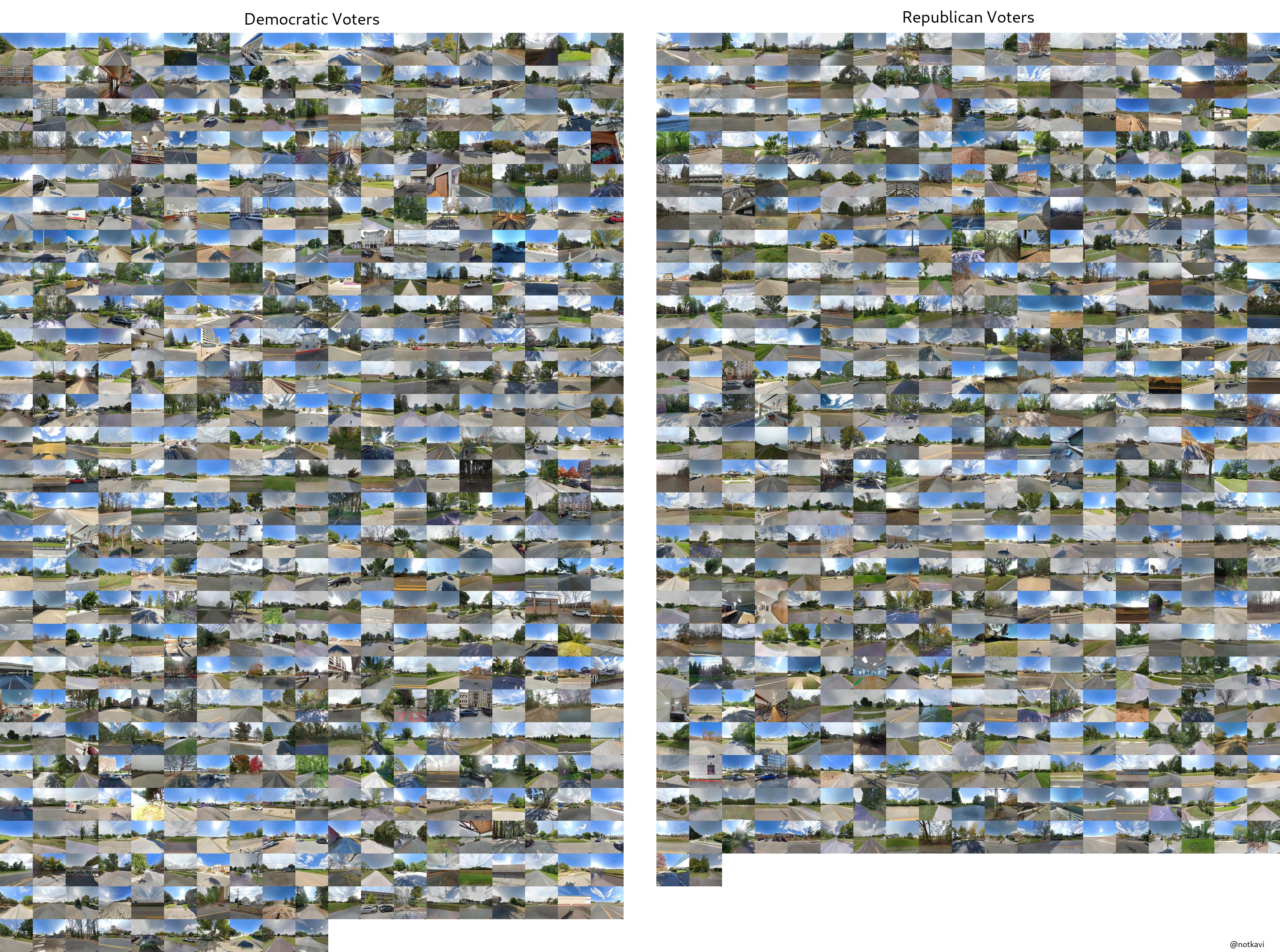
Election maps tend to obscure a couple things that I think are interesting about American elections.
First, about 33% of Trump supporters, and about 30% of Biden supporters lived in precincts that voted for the other party, so show up in the other party’s color on the map!
Second, the map tends to overstate the number of people who live in purely rural areas.
The combination of these two effects leads to in my view a fairly big distortion of our pictures of blue and red America, but especially red America, which people begin to picture as entirely middle-of-nowhere rural areas.
Instead, here’s a sampling of 1000 voters and what their neighborhoods look like. This has the benefit of giving you a picture of what Biden’s America and Trump’s America look like: not two disjoint nations, but two overlapping and intertwined distributions. You can click each dot to jump down to the voter represented by the dot.
Voting is Rational
A common refrain in politics-adjacent discourse is “why bother voting? there’s no chance your individual vote will affect the outcome of the election!” This concept is often conceptualized in political science as the Paradox of Voting. However, with a few simple assumptions, the paradox disappears.
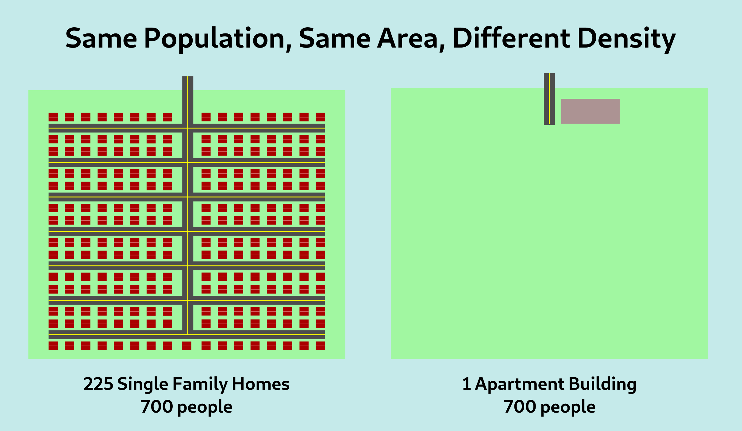
You're calculating population density incorrectly
The question “how do you calculate population density?” sounds like the kind of thing you’d see on a third grade pop quiz. Obviously, you would calculate it in the same way you would calculate any other type of density: you take the feature of interest and its population, and divide by area.
The issue is that this approach assumes that every part of the region of interest is equally valuable.
Why do we care about density?
For example, consider the following two islands:
BAN ALL AMBIGUOUS MATHEMATICAL EXPRESSIONS
If you’re on twitter or Facebook you’ve probably seen this expression (or a variant with different numbers) before
6 ÷ 2(1+2)
The question that goes with it is “can you solve this?” and there’s usually a massive debate among people in the comments about whether the answer is 9 (corresponding to dividing first then multiplying by (1+2)) or 1 (corresponding to multiplying first to get 6 then dividing).
Setting the actual size of figures in matplotlib.pyplot
Let’s say you want to set the size of a figure in matplotlib, say because you want the captions to match the font size on a poster (this came up for me recently). However, you might find yourself with kinda a weird problem.
Directly setting the size of a figure
Setting the actual size of figures in matplotlib.pyplot is difficult. Setting the size of a figure as so
plt.figure(figsize=(5, 2.5))
plt.plot([1, 2, 3], [4, 5, 6])
plt.xlabel("x label")
plt.ylabel("y label")
plt.savefig("direct.png")
print(imread("direct.png").shape) # outputs (250, 500, 4)
Understanding Python's interactive mode
The Python interepreter has this convenient feature that when you type something simple onto the interpreter, it spits that value back out at you, so you can copy/paste it back as a value.
But with convenience often comes complexity, let’s look at how this feature works!
Simulationism: Beyond the Matrix
Simulationism is a fairly popular concept. There are many who subscribe to it: from those who use it as a thought experiment to argue against undisprovable theories to those who actually believe we are in a simulation since almost all universes should be simulations. Despite the disparate uses for simulationism, it is generally viewed as a fairly banal concept: the universe is a simulation, and that means absolutely nothing, practically speaking.
However, lurking beneath the seeming simplicity of the idea lies a far more radical set of implications.
Lists and Nonlocal in Python
Mutable closures
A closure is a function with a parent frame that contains some data. If the parent frame can be modified, the function is said to be mutable.
For example, take the following doctest:
>>> c, d = make_counter(), make_counter()
>>> c()
0
>>> c()
1
>>> c()
2
>>> [c(), d(), d(), d(), c()]
[3, 0, 1, 2, 4]
The c is called multiple times and returns a different value every time; but its state isn’t global as there is the d function which also counts up but on its own tineline.
The Python programming language allows for the creation of mutable closures in two different ways: one that is traditionally considered “functional” and one that is traditionally considered “object-oriented”. Let’s take a look at them now:
Confirming that timezones exist with minimal trust
I was listening to an episode of Oh No, Ross and Carrie! about Flat Earth and it struck me that if you believe the world is conspiring against you, it’s practically quite difficult to prove almost anything. Now one thing that most Flat Earthers do seem to accept is that when its day in one part of the planet, it’s night in another part.
However, let’s say someone denied this. How would you prove it, with the minimum amount of trust?
Infix Notation in Scheme
Scheme is well known as a very simple programming language. The general concept behind scheme is that it is composed of S-expressions, or expressions of the form (operator operand1 operand2 ... operandn), which can be nested.
This makes scheme relatively simple to parse and evaluate, however it does lead to some strange compromises on the style of programming. For example, rather than writing 12 * (2 + 3), you have to write (* 12 (+ 2 3)). And in a way, this is elegant in its simplicity.
But simplicity is overrated.
(Mini) Scheme in 50 Lines
The scheme language is a programming language that is unique for being easy to parse. Every construct in scheme is of the form
(keyword arg1 ... argn)
Our Subset
We will start with some standard scheme expressions, which you can think about as being analogous to certain patterns in Python. For example instead of writing a + b, you write (+ a b), where + is just the name of a function. Similarly, instead of writing lambda x: x * 2 for the doubling function, you write (lambda (x) (* 2 x)). Just lambdas and function application are enough to perform any calculation, but we add a few more features for clarity: instead of x = y we write (define x y), instead of x if y else z we write (if y x z) and instead of writing
x = f(y)
return x
we write (begin (define x (f y)) x). The real scheme language has many more constructs, including ones that simulate python’s def statements, and some unique ones that allow you to assign variables in a local frame, simulate elif trees, have short-circuited and/or constructs, or even define your own language constructs. For brevity, we will stick to this subset, which is still very powerful.
The Efficiency Gap Makes No Sense (but all metrics show Republicans are better at gerrymandering)
Cracking, Packing, and Wasted Votes
The efficiency gap is a technique for measuring the level of gerrymandering in a state. Gerrymandering generally takes the form of what’s known as “cracking and packing.” Cracking is the process of taking a district with a majority of the opposing party and splitting it into two in which the party has a minority in each, thus denying your opponent that seat. However, this isn’t always possible because your opponent might have too many votes in a given area. To reduce the remaining number of votes your opponent has while minimizing the number of seats they have, you can use a technique called packing, in which you create a district in which your opponent can win by a huge margin.
To measure both cracking and packing, we can use the concept of a wasted vote. A wasted vote is any vote that did not contribute to the victory. There are two kinds of wasted votes, cracked waste and packed waste. A cracked wasted vote for party X is any vote in a district party X has lost. A packed wasted vote is any vote for party X over 50% in a district party X has won.
For example, let’s say that there are just two parties1 and 1000 voters in a district. The number of wasted votes for X in terms of the number of votes for X is as such:
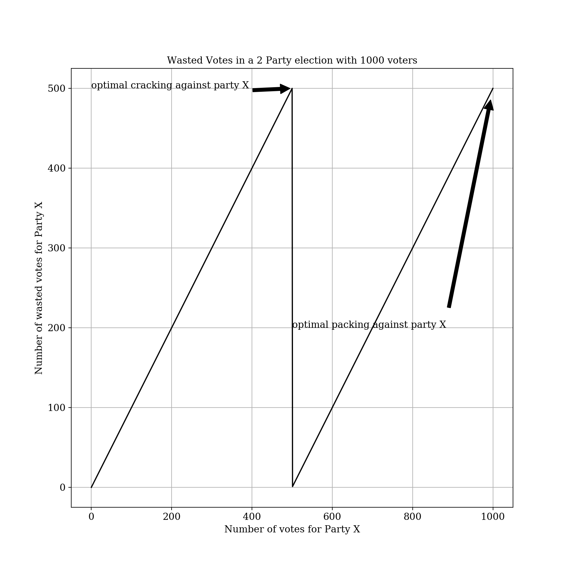
-
The United States has two political parties. A vote for the Green, Libertarian, or American Independent Party is a wasted vote. But if you’re voting for the AIP (the party that nominated Wallace), you should waste your vote, so I guess I’m fine if you vote for the AIP. ↩
How You Get Homeopathy
Homeopathy is a system that has two primary claims. The first is the law of similars. It says that a dilute solution of a substance cures the ailment caused by a concentrated solution of the same substance. The second is the law of dilution, which says that the more dilute a homeopathic preparation is, the stronger its effect.
The second theory is the one people tend to focus on because it is clearly incorrect. The anti-homeopathy \(10^{23}\) campaign is named after the order of magnitude of Avogadro’s number, that is the number of molecules of a substance in a 1M solution of a substance (typically a fairly strong solution, 1M saltwater is 5 teaspoons of salt in a liter of water). If you dilute by more than that amount, and many “strong” homeopathic preparations do, then with high probability you literally have 0 molecules of the active ingredient in your preparation. As the \(10^{23}\) campaign’s slogan makes clear, “There’s nothing in it” and homeopathic medicines are just sugar pills.
What is NP?
What is P?
This seems like a silly question. This question seems easily answered by the surprisingly comprehensible explanation on P’s Wikipedia page:
It contains all decision problems that can be solved by a deterministic Turing machine using a polynomial amount of computation time
OK, so it’s the set of all decision problems (yes-or-no questions) that are \(O(n^k)\) for some integer \(k\). For example, sorting, which is \(\Theta(n \log n)\) is P, since it’s also \(O(n^2)\).
But let’s go for an alternate definition. Let’s take a C-like language and get rid of a bunch of features: subroutine calls, while loops, goto, for loops with anything other than i < n in the second field (where n is the length of the input), and modifying the for loop variable within the loop. Effectively, this language’s only loping construct is for(int varname = 0; varname < n; varname++) {/* Code that never modifies varname */}. Let’s call this language C-FOR.
Storing Data With the Circle-Tree
The Pair Abstraction
Computers need some way to store information. More specifically, we want to be able to store multiple pieces of data in one place so that we can retrieve it later. For now, we’ll look at the simplest way of storing data, a pair.
To express the concept of a “pair”, we need three machines.
- A way to put two things together (construction, or “C” for short)
- A way to get the first element (first, or “F” for short)
- A way to get the second element (second, or “S” for short)
Circle-Tree as a Calculator
Using Circle-Tree Drawings as a Calculator
So this isn’t just a procrastination game for doodling when you’re bored (and have a lot of colored pencils, for some reason). We can use circle-tree as a way to express math!
Numbers
For math, the first thing we need are numbers. I’m just going to draw some pictures which are defined to be the numbers. We don’t worry too much about whether they are “really” numbers or not in the way that we don’t worry about whether “102” or “CII” is a better way to explain the concept of “how many cents in a dollar plus how many hands a person has”ness.1
So this is 0:

-
Although, off the record, for doing math CII is a terrible way of representing 102. ↩
Introducing the Circle-Tree System
If you want to follow along on paper, you’ll want some colored pencils. Like at least 5 colors, not including a pencil to draw links.
Circtrees
In any case, we’ll call the diagrams we’re interested in “circtrees.”1 Circtrees can be constructed in one of three ways.
1. Dots
A dot of any color is a circtree. Here are some examples2:

Counting Monoids
What’s a Monoid?
A monoid is a set \(M\) with an identity element \(e : M\) and an operation \(* : M \to M \to M\), where we have the laws:
- \(x * e = x\)
- \(e * x = x\)
- \(x * (y * z) = (x * y) * z\)
We write a monoid as a tuple \((M, e, * )\). Some example monoids (written in pseudo-Haskell) are
(Int, 0, (+))
(Int, 1, (*))
(Bool, True, (||))
((), (), \x y -> ())
([a], [], (++))
The Porus Mirror Problem, Part 2
Propagation
From last time, we know the quantity of light that escaped at each location and direction around the unit circle. We want to find how this translates into quantities of light at any point away from the circle. This situation can be modeled as so:
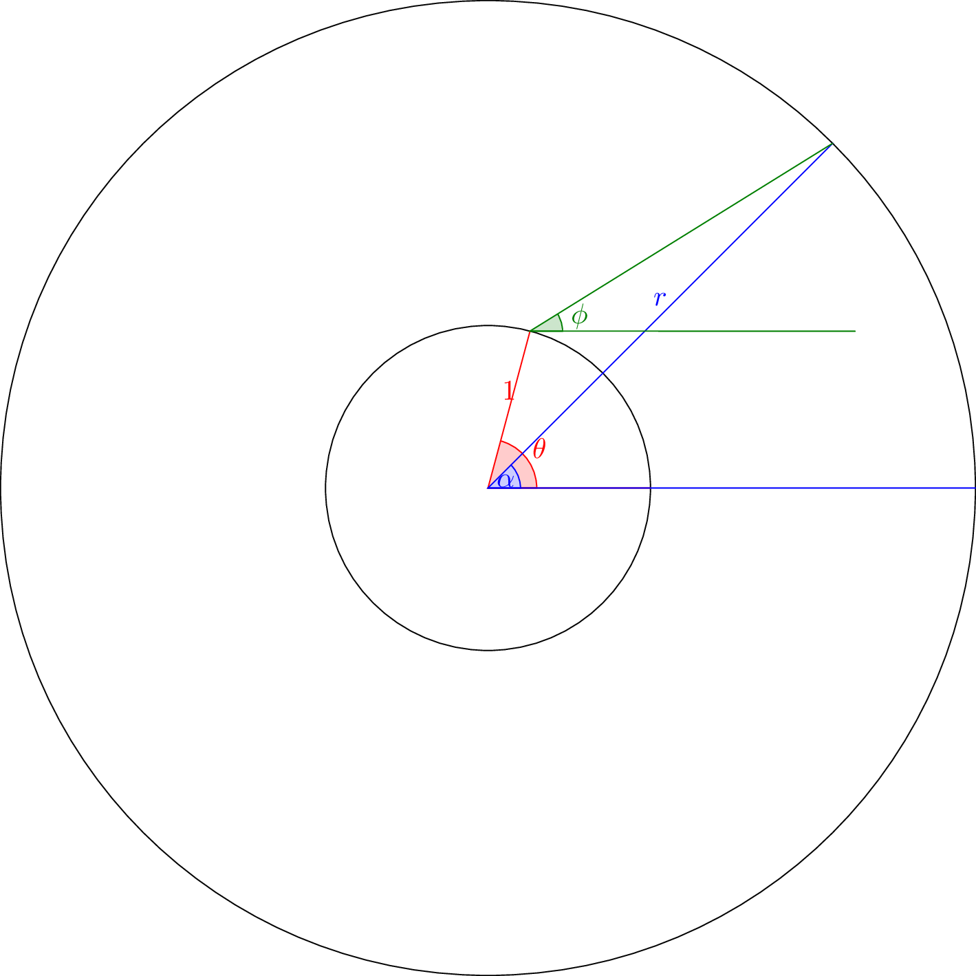
The Porus Mirror Problem, Part 1
The porus mirror problem
I’m pretty sure I came up with this problem on my own, but I’m not sure if its an existing problem under a different name. Anyway, the situation is as such:
- We have a very short cylindrical tube. In fact, we’ll ignore the third dimension and just use a circle. For simplicity, we’re using units such that the radius is 1.
- The tube is filled with a gas that emits corpuscles in one large burst. We assume a large enough number that we can model them continuously. We additionally assume that the emmissions are uniform in location and direction.
- The tube itself is semitransparent, with transparency determined by a function \(t: [0, 2\pi] \to [0, 1]\) of angle around the circle. Any light that does not pass through is reflected across the normal.
We wish to calculate at each point along the surface of the tube what is the total quantity of light emitted in each direction, from which we can easily calculate the light pattern this system will cast on any shape outside.
Dependent Types and Categories, Part 1
So I’ve been trying to go through Category Theory for Scientists by writing the functions as code. So I obviously decided to use Haskell. Unfortunately, I ran into a wall: Haskell is actually pretty bad at representing categories.
Haskell is a Category
Now, at first this was incredibly surprising. Frankly, I had started learning about category theory because of its association with Haskell. Unfortunately, I didn’t realize that Haskell isn’t category theory, it’s a category.
For instance, look at this definition of a category in math:
Chaos, Distributions, and a Simple Function
\(\newcommand{\powser}[1]{\left{ #1 \right}}\)
Iterated functions
The iteration of a function \(f^n\) is defined as:
\[f^0 = id\] \[f^n = f \circ f^{n-1}\]
For example, \((x \mapsto 2x)^n = x \mapsto 2^n x\).
Most functions aren’t all that interesting when iterated. \(x^2\) goes to \(0\), \(1\) or \(\infty\) depending on starting point, \(\sin\) goes to 0, \(\cos\) goes to something close to 0.739. \(\frac{1}{x}\) has no well defined iteration, as \((x \to x^{-1})^n = x \to x^{(-1)^n}\) which does not converge.
Haskell Classes for Limits
OK, so the real reason I covered Products and Coproducts last time last time was to work toward a discussion of limits, which are a concept I have never fully understood in Category Theory.
Diagram
As before, we have to define a few preliminaries before we can define a limit. The first thing we can define is a diagram, or a functor from another category to the current one. In Haskell, we can’t escape the current category of Hask, so we instead define a diagram as a series of types and associated functions. For example, we can define a diagram from the category \(\mathbf 2\) containing two elements and no morphisms apart from the identities as a pair of undetermined types.
A diagram from the category \(\mathbf 2*\), a category containing two elements and an arrow in each direction (along with the identities), (this implies that the two arrows compose in both directions to the identitity):
Haskell Classes for Products and Coproducts
Product Data Structures
Product Types are a familiar occurrence for a programmer. For example, in Java, the type int \(\times\) int can be represented as:
class IntPair {
    public final int first;
    public final int second;
    public IntPair(int first, int second) {
        this.first = first;
        this.second = second;
    }
}
Monoids, Bioids, and Beyond
Two View of Monoids.
Monoids
Monoids are defined in Haskell as follows:
class Monoid a where
    m_id :: a
    (++) :: a -> a -> a
Monoids define some operation with identity (here called m_id). We can define
the required laws, identity, and associativity, as follows:
monoidLaw1, monoidLaw2 :: (Monoid a, Eq a) => a -> Bool
monoidLaw1 x = x ++ m_id == x
monoidLaw2 x = m_id ++ x == x

monoidLaw3 :: (Monoid a, Eq a) => a -> a -> a -> Bool
monoidLaw3 x y z = (x ++ y) ++ z == x ++ (y ++ z)
Nontrivial Elements of Trivial Types
We know that types can be used to encode how to make useful data structures.
For example, a vehicle can be encoded as:
data Vehicle = Car { vin :: Integer, licensePlate :: String }
        | Bike
In this case, valid values include cars with VINs and LPNs, or Bikes, which have neither of these data points.
However, some data types can seem far less useful.
The Autogeneration of Landscapes
OK, so a break from theory and CS, and to applications. How do we produce reasonably realistic landscapes using differential equations?
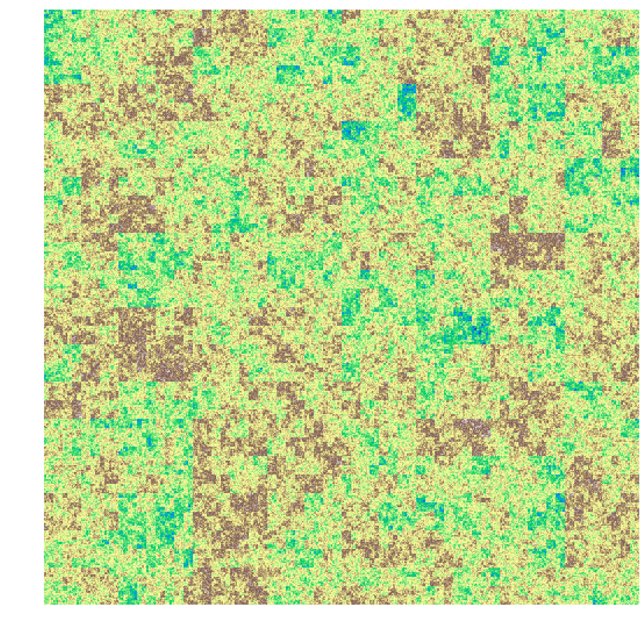
Mountains and Valleys
To simulate mountains and valleys, we can use a fairly simple algorithm that adds a random amount to a region, then recursively calls itself on each quadrant of the region. Afterwards, an image generally looks something like:
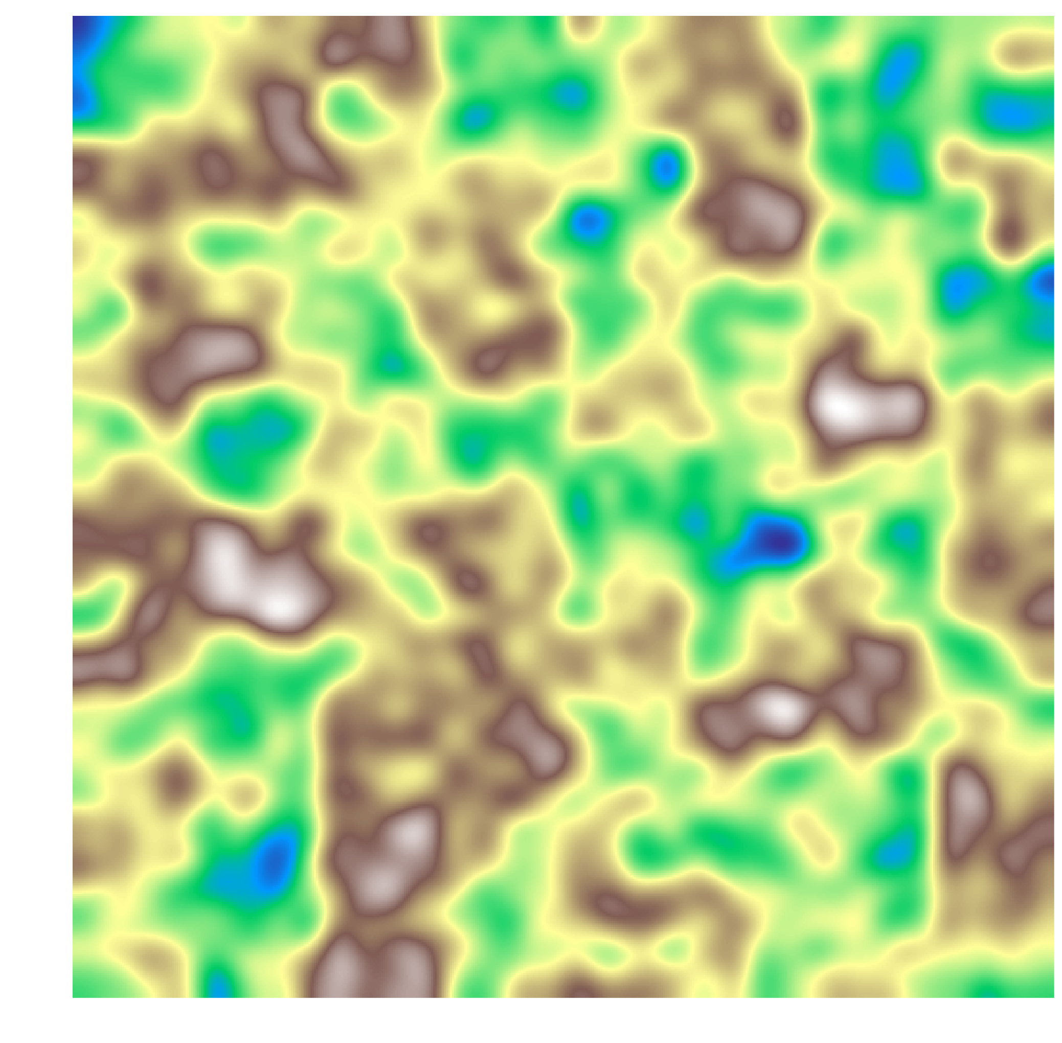
We can apply a Gaussian blur to the image to get a reasonably realistic depiction of mountains and valleys.
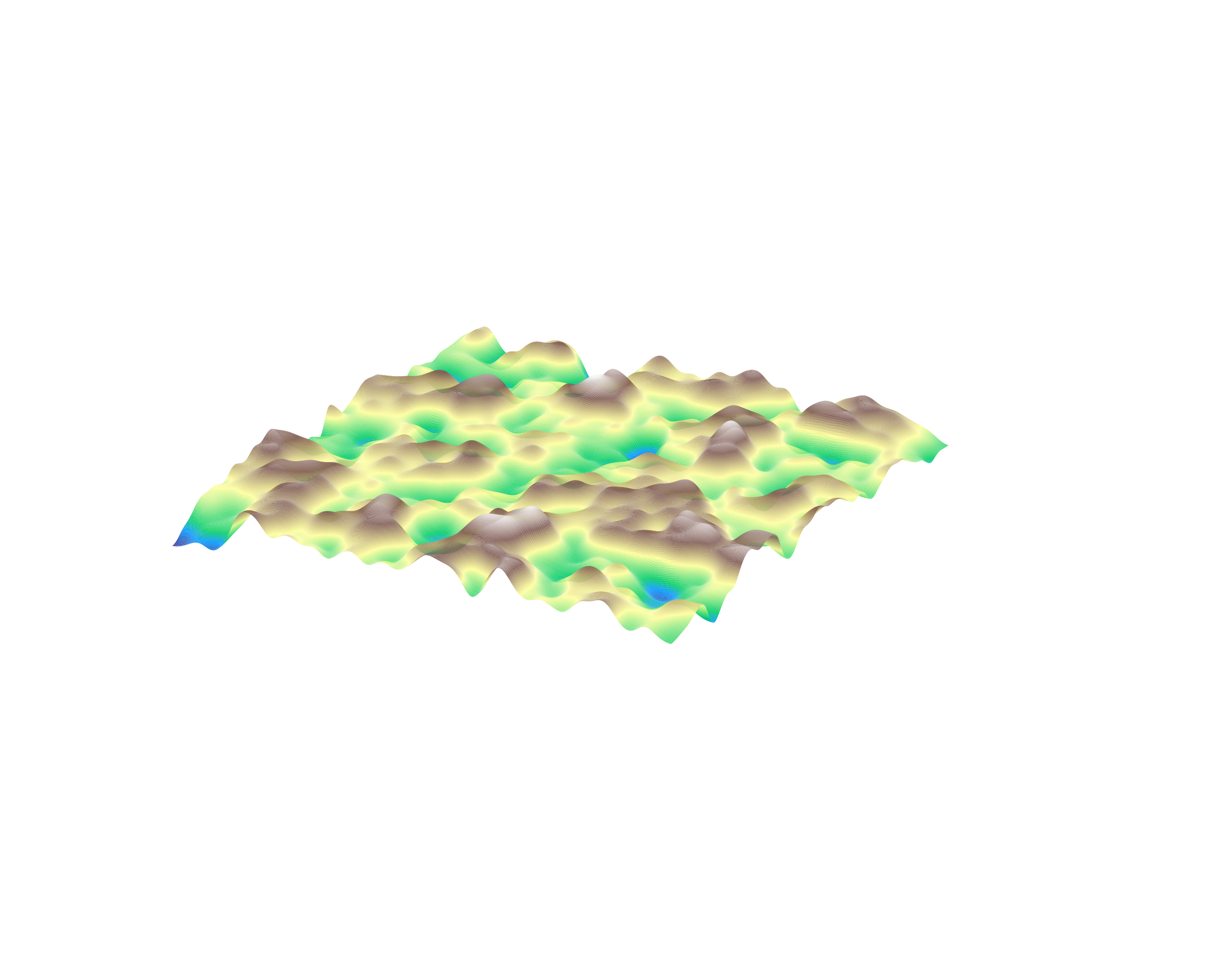
We can define the elevation as a function \(E(x, y, t)\). Representing this as a landscape:
C-Style Pointer Syntax Considered Harmful
Declaration Follows Use
In C, a pointer to int has type int*, but really, this isn’t the right way of looking at it. For example, the following declaration:
int* x, y;
creates x of type int* and y of type int.
The Triviality Norm
Feynman famously said that to a mathematician, anything that was proven was trivial. This statement, while clearly a lighthearted dig at mathematics, it does have a striking ring of truth to it.
Logical Implication
In logic, there is the concept of implication. The idea is that if \(B\) is true whenever \(A\) is true we can say that \(A \implies B\). This makes sense for statements that depend on a variable. For example, we can say that \(x > 2 \implies x > 0\).
A Monadic Model for Set Theory, Part 2
\(\newcommand{\fcd}{\leadsto}\)
Last time, we discussed funcads, which are a generalization of functions that can have multiple or no values for each element in their input.
Composition of Funcads
The composition of funcads is defined to be compatible with the composition of functions, and it takes a fairly similar form:
\[f :: Y \fcd Z \wedge f :: X \fcd Y \implies \exists (f \odot g :: X \fcd Z), (f \odot g)(x) = \bigcup_{\forall y \in g(x)} f(y)\]
In other words, map the second function over the result of the first and take the union. If you’re a Haskell programmer, you probably were expecting this from the title and the name “funcad”: the funcad composition rule is just Haskell’s >=>.
A Monadic Model for Set Theory, Part 1
\(\newcommand{\fcd}{\leadsto}\)
Solving an Equation
A lot of elementary algebra involves solving equations. Generally, mathematicians seek solutions to equations of the form
\[f(x) = b\]
The solution that most mathematicians come up with to this problem is to define left and right inverses: The left inverse of a function \(f\) is a function \(g\) such that \(g \circ f = \mathrm {id}\). This inverse applies to any function that is one-to-one. There is also a right inverse, a function \(g\) such that \(f \circ g = \mathrm {id}\) For example, the left inverse of the function
\[x \mapsto \sqrt x :: \mathbb R^+ \rightarrow \mathbb R\]
is the function
\[x \mapsto x^2 :: \mathbb R \rightarrow \mathbb R^+\]
What is Category Theory?
\(\newcommand{\mr}{\mathrm}\) So, I was reading Category Theory for Scientists recently and kept having people ask me: What is category theory? Well, until I hit chapter 3-4, I didn’t really have an answer. But now I do, and I realize that to just understand what it is doesn’t really require understanding how it works.
Sets and functions
So, set theory is all about sets and functions. Why are we talking about set theory and not category theory, you may ask? I’ll get to category theory eventually, but for now, let’s discuss something a little more concrete.
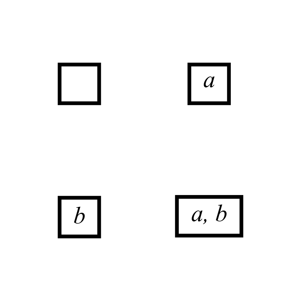
Let’s look at subsets of the set \(\{a, b\}\). We have the possibilities, which we name Empty, A set, B set, Universal set:
\[E = \{\}, A = \{a\}, B = \{b\}, U = \{a, b\}\]
Stupid Regex Tricks
Regexes, the duct tape of CS
Regexes are truly amazing. If you haven’t heard of them, they are a quick way to find (and sometimes replace) some body of text with another body of text. The syntax, while it has its critics, is generally pretty intuitive; for example a zip code might be represented as
[0-9]{5}(\s*-\s*[0-9]{4})?
which is read as “a five digit code optionally followed by a spaced dash and a four digit code”. Some whitespace and named groups might help the reading (use COMMENTS mode when parsing)
(?P<main_code>
    [0-9]{5}
)
( # optional extension
    \s*-\s*     # padded dash
    (?P<optional_extension>
        [0-9]{4}
    )
)?
Dictp Part 2
OK, so to continue the Dictp saga, some syntactic sugar.
References to local variables.
The parser can be enhanced by rewriting anything that isn’t a built-in command or a string with a lookup to __local__.
E.g.,
a\(\mapsto\)__local__['a']0 = 1\(\mapsto\)__local__['0'] = __local__['1']0?\(\mapsto\)__local__['0']?'0'\(\mapsto\)'0'
Dictp Part 1
So, a friend and I (I’m going to protect his anonymity in case he doesn’t want to be associated with the travesty that is what we ended up thinking up) were discussing ridiculous ideas for programming languages: you know the deal, writing C interpreters in Python, using only integers to represent everything, etc.
One idea, however, seemed a little less ridiculous to us (OK, just to me): a language in which there are two data types: Dictionary and String.
Infsabot Strategy Part 2
OK, so to continue our Infsaboting.
Correction
I made a mistake last time. I included SwitchInt, a way to switch on values of ExprDir, which is ridiculous since an ExprDir can only be constructed as a constant or an if branch to begin with.
So just imagine that I never did that.
Guess and Check
OK, so how should our AI construct these syntax trees? At a very high level, we want to be able to 1) assess trees against collections of trees and 2) modify them randomly. We can represent this as a pair of types:
asses :: [RP] -> RP -> Double
modify :: RP -> StdGen -> (RP, StdGen)
I think the implementation of asses should be pretty clear: simply find the win rate (given that we can simulate an unlimited number of games).
Modify, on the other hand, is a little more complicated. There are a few ways a tree can be modified:
- Modify the value of a constant to be something else.
- Modify the value of a field to point to something else or a field
- Add leaves to the tree
- Remove leaves as a simplification step
Infsabot Strategy Part 1
OK, so what is this Infsabot? Infsabot is a game I designed for people to write programs to play. Basically, it’s like chess, except where each piece acts independently of each other.
The Game
There is a square board where each square is either empty or contains material. The game pieces, robots, require material to stay alive and perform tasks. At each turn, every robot reports which of the following it wants to do:
- Noop: The robot does nothing
- Die: The robot dies
- Dig: The robot digs to try to extract material
- Move: The robot can move in one of the four compass directions
- Fire: The robot can fire a quick-moving projectile (e.g., travel time = 0) in a compass direction
- Message: The robot can send a quick-moving message in a compass direction
- Spawn: The robot can create a new robot with its own initial material and appearance
To decide what to do, a robot has access to two things:
- A picture of the positions around it, to a given distance
- Whether or not the spot contains material
- Whether or not the spot contains a robot, and it’s appearance (not it’s team)
- A snapshot of its own hard drive, which is a massive relational database between Strings and Strings
- A list of all messages received
What's a number?
OK, so a bit of a silly question. Of course, we all know what numbers are. But humor me, and try to define a number without using “number”, “quantity”, or anything that refers back to a number itself.
But, before we learn numbers, we have to first understand something simpler: counting. Couldn’t we define numbers in terms of counting? Well, yes, otherwise I wouldn’t be writing this article.
Now, to not end up with a forty page book, I’m only going to go over how to define the whole numbers (I’m going to ignore negative integers, fractions, \(\pi\), etc.)
Recursivized Types
So, a short break from \(\varepsilon—\delta\).
Anyway, I’m going to look at Algebraic types in this section. Specifically, I am going to use Haskell types.
The provided code is all actual Haskell, in fact, I’m going to have to de-import the standard libraries because some of this is actually defined there. You can find all the code here
Who Needs Delta? Defining the Hyper-Real Numbers
\(\renewcommand{\ep}{\varepsilon}\) \(\renewcommand{\d}{\mathrm d}\)
In high school Calculus, solving differential equations often involves something like the following:
\[\frac{\d y}{\d x} = \frac{y}{x}\]
\[\frac{\d y}{y} = \frac{\d x}{x}\]
\[\int \frac{\d y}{y} = \int \frac{\d x}{x}\]
\[\log y = c + \log x\]
\[y = kx\]
Now, I don’t know about anyone else, but this abuse of notation really bothered me at first. Everyone knows that \(\d x\) isn’t an actual number by itself, but we seem to use it all the time as an independent variable.
Ancient Greek Abstract Algebra: Introduction
Note: I’ve put the Ancient Greek Abstract Algebra series on hold for now. Please take a look at some of my other post(s).
Modern constructions of \(\mathbb{N}\)
The natural numbers are taught to children as a basic facet of mathematics. One of the first things we learn is how to count. In fact, the name “Natural Numbers” itself implies that the natural numbers are basic.
However, modern mathematicians seem to have trouble with accepting the natural numbers as first class features of mathematics. In fact, there are not one but two common definitions of the naturals that can be used to prove the Peano Axioms (the basic axioms from which most of number theory can be proven).